


It's an amazing feeling to wake up to the sight of Sun gazing through the windows with the Spring just around the corner. One feels so much more energetic, and willing to productively fulfill your day in this great atmosphere :D
So I thought to myself the other day: "Why not use this energy and try to make something meaningful today - that would potentially sharpen my coding skills?" I've been recently diving deep into Computer Vision, and been coding a lot image classification architectures using this great framework - TensorFlow.
I found this dataset from Kaggle which I'll use in this notebook/project:
Kaggle: National Flowers - Shahidul Islam Zahid
Insight into Images
First, I'd like to know how many images there are, for each class in the training dataset, so let's find out.
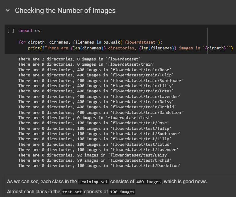
Looks like the training dataset seems pretty balanced with exactly 400 images per each class. What would be even better to know, though, is how our training images of the flowers exactly look like so we can know if there is any noise in the training dataset :D Let's write a function that will visualize a random image for us.
# Necessary imports
import random
import matplotlib.pyplot as plt

def view_random_image(dir, class_name=None):
    """
    Takes a directory, and a desired class, and displays an image of a random flower belonging to the chosen class

    Args:
        dir (str): The directory with images (can display test images as well).
        class_name (str): The desired class, from which to display a flower. By default: None, if set to None, then a random class will be chosen.
    """
    # Define the path
    if class_name:
        full_path = dir + "/" + class_name
    else:
        class_name = random.choice(class_names)
        full_path = dir + "/" + class_name

    # Get the random image & define full image path
    rand_img = random.choice(os.listdir(full_path))
    full_img_path = full_path + "/" + rand_img

    # Plot the random image
    img = plt.imread(full_img_path)
    plt.axis(False)
    plt.title(class_name)
    plt.imshow(img)
I set it up so that you can visualize images from any desired path (meaning validation/test split as well). Now let's see how (if :D) the function works!
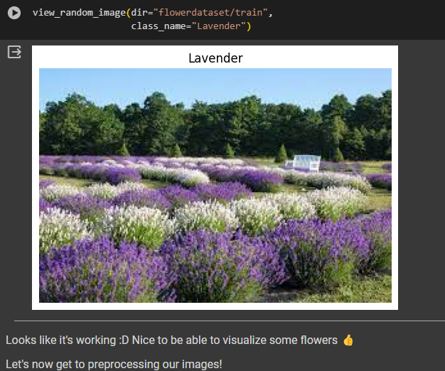
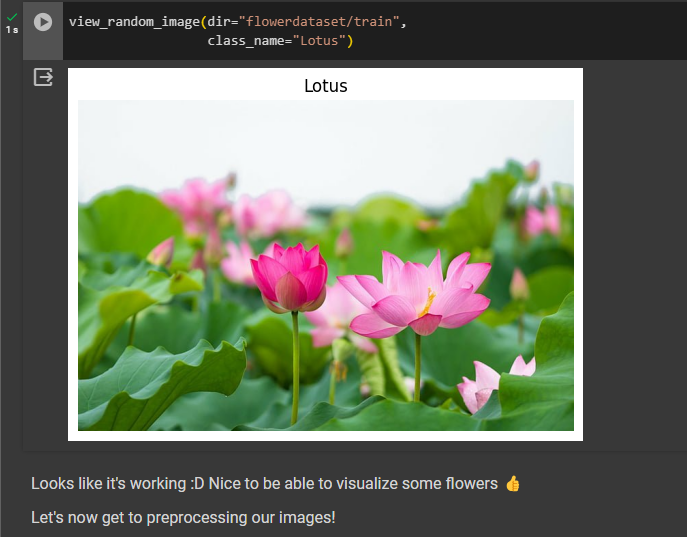
Yup, looks like it works flawlessly. With the Spring lurking right outside my window, I could really look at the flower images all the time hahaha - it really is addicting...
Preprocessing the Images
Even though we (as humans) prefer the flower images to be in the form of flower images :D, our neural net would rather that the images were:
in the numerical form,
represented as Tensors,
preferably scaled.
We'll also transform the images into batches - each of size 32. Let's take care of that! Now here's some custom function I made to conveniently preprocess the images.
from tensorflow.keras.preprocessing.image import ImageDataGenerator

# Define paths
TRAIN_PATH = "flowerdataset/train/"
TEST_PATH = "flowerdataset/test/"

# Define data generators
train_datagen = ImageDataGenerator(rescale=1/255.)
test_datagen = ImageDataGenerator(rescale=1/255.)

# Actual training/test datasets
print("Training images:")
train_data = train_datagen.flow_from_directory(directory=TRAIN_PATH,
                                               target_size=(224, 224),
                                               class_mode="categorical",
                                               batch_size=32)

print("Test images:")
test_data = test_datagen.flow_from_directory(directory=TEST_PATH,
                                             target_size=(224, 224),
                                             class_mode="categorical",
                                             batch_size=32)
Modelling the Data
Now the real fun begins! :D For this purpose I'll utilize transfer learning. Since I haven't yet done any research about fine-tuning... I guess feature extraction will have to suffice for now :D
I'll try out 3 popular architectures of Convolutional Neural Networks, namely:
MobileNetV2
ResNetV2
EfficientNetB0
If I were to put my money on any of these architectures, it'd be EfficientNet... Let's try all three architectures nonetheless :D
Custom TensorBoard Callback Function
Let's first create a little custom function that will help us track our experiments on TensorBoard.
import datetime
import tensorflow as tf

def create_tensorboard_callback(dir_name, experiment_name):
    """
    Takes the desired directory name, experiment name and saves TensorBoard logs over there.

    Args:
        dir_name (str): The desired directory.
        experiment_name (str): The desired name of an experiment with model.

    Returns:
        tensorboard_callback instance.
    """
    # Define the logging directory and return the callback
    log_dir = dir_name + "/" + experiment_name + datetime.datetime.now().strftime("%H-%M-%S-%d-%m-%Y")
    tensorboard_callback = tf.keras.callbacks.TensorBoard(log_dir=log_dir)
    print(f"Saving logs to {log_dir}")
    return tensorboard_callback
I always (try to remember to :D) include the docstring for my custom functions so that the persom on the otherside can understand it more quickly. I believe a great intercommunication can work wonders :D
Custom Loss & Accuracy Curve Function
I thought it would be a not bad idea to quickly visualize loss and accuracy curves for our models without having to launch up TensorBoard every time so let's write a custom function for this purpose.
def plot_loss_acc(history, epochs=5):
    """
    Takes a history instance, and the number of epochs. Produces 2 plots of loss and accuracy (separately).
    """
    # Define vars
    loss = history.history["loss"]
    val_loss = history.history["val_loss"]
    accuracy = history.history["accuracy"]
    val_accuracy = history.history["val_accuracy"]
    epochs = range(len(history.history["loss"]))

    # Plotting loss
    plt.plot(epochs, loss, label="training_loss")
    plt.plot(epochs, val_loss, label="validation_loss")
    plt.title("Loss")
    plt.xlabel("Epochs")
    plt.legend()

    # Plotting accuracy
    plt.figure()
    plt.plot(epochs, accuracy, label="training_acc")
    plt.plot(epochs, val_accuracy, label="validation_acc")
    plt.title("Accuracy")
    plt.xlabel("Epochs")
Custom Function to Create Models
I'll functionize this process as well, so that we won't have to write every single time 'tf.keras.Sequential([........]) :D
# Defining Nets' URLs
MOBILENET_V2_URL = "https://www.kaggle.com/models/google/mobilenet-v2/frameworks/TensorFlow2/variations/100-224-feature-vector/versions/2"
RESNET_V2_URL = "https://www.kaggle.com/models/google/resnet-v2/frameworks/TensorFlow2/variations/152-feature-vector/versions/2"
EFFICIENTNET_V2_URL = "https://www.kaggle.com/models/google/efficientnet-v2/frameworks/TensorFlow2/variations/imagenet21k-b0-feature-vector/versions/1"
NUM_CLASSES = 9
import tensorflow_hub as hub

def create_model(model_url):
    """
    Takes model's URL from Kaggle and creates an uncompiled Keras Sequential model with it.

    Args:
        model_url (str): A weblink of the desired model to utilize.

    Returns:
        An uncompiled Keras Sequential model with `model_url` as feature extraction
        layer, and Dense layer with `NUM_CLASSES` output neurons.
    """
    model = tf.keras.Sequential([
        hub.KerasLayer(model_url,
                       trainable=False, # feature extraction
                       name="feature_extraction_layer",
                       input_shape=(224, 224, 3)),
        tf.keras.layers.Dense(NUM_CLASSES, activation="softmax", name="output_layer")
    ])
    return model
MobileNetV2 & ResNetV2 Experiment Results
I wonder if there will be a fierce competition between MobileNetV2 and ResNetV2 :D Let's see which one beats the other one.
I have included training & validation results after building, compiling & fitting both models on the training data & validating on the test data (since the dataset from Kaggle didn't include a validation set - I decided to validate on the testing data...). Maybe an interesting follow-up would be to create my own validation test - split from the already existing training set? We'll train all 3 models for 5 epochs. Enough talking:
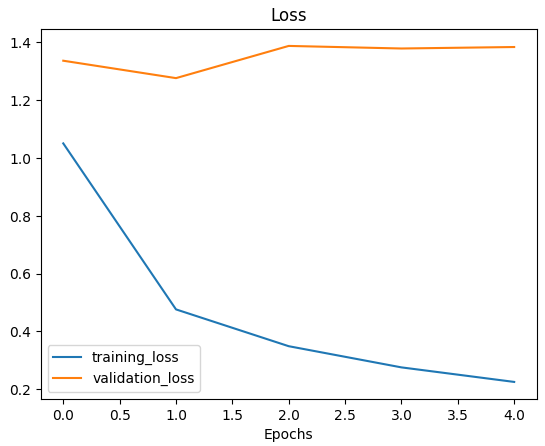
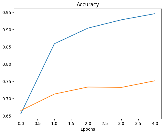
MobileNetV2 Results:
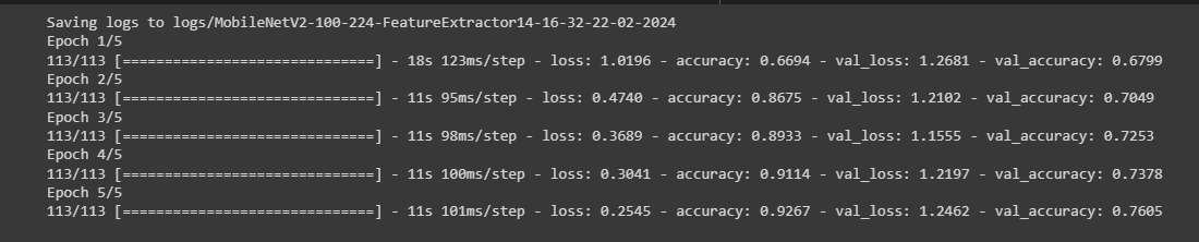
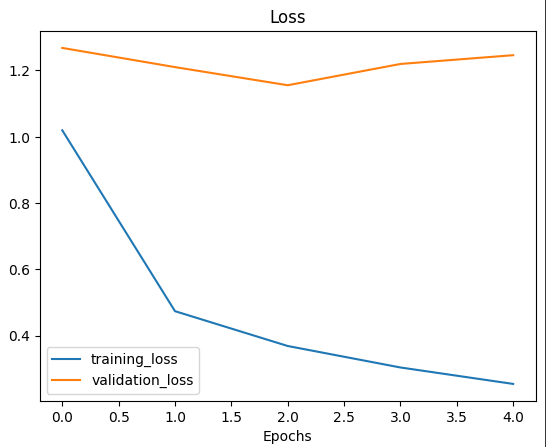
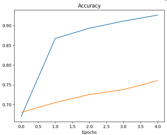
Woohoo, great to see my custom function up & running flawlessly :D The validation loss seems to start plateauing after epoch 2. The validation accuracy also seems to plateau at around epoch 4, which hints our model is overfitting.
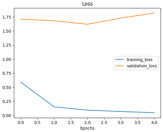
Alright let's now check ResNetV2 Experiment Results:
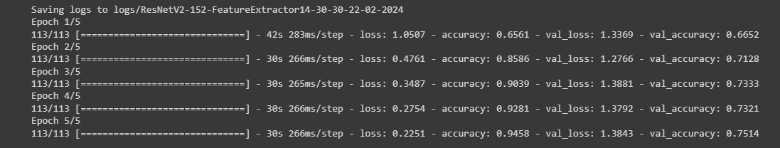
Oooh, apparently our ResNetV2 model starts to overfit even faster at epoch 1. The models' evaluations are somewhat comparable. ResNetV2 model started off with a slightly worse training accuracy and validation accuracy, and also finished training with a slightly 'worse' validation losses and accuracies. Let's show them both how it's done using EfficientNetB0 Architecture :D.
EfficientNetB0 Experiment Results:
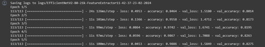
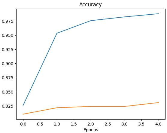
Note: The blue trend represents the training accuracies, while the orange trend represents the validation accuracies. I thought I added both plotting legends but apparently I had forgotten to, so here's a little clarification :D
Woow - watch that! Our EfficientNetB0 architecture model started off with a training accuracy of ~0.84 (almost 20 percentage points higher than the MobileNetV2 and the ResNetV2 (!)), and with a validation accuracy of ~0.8. It started overfitting rather quickly at epoch 2 - but this is great news anyway!
(I guess my bet on the EfficientNet was successful hehe 🤑)
I believe this model will be more than enough for a few predictions on some custom images :D Cause this is where the most fun is, right? Seeing our model do well on validation/test data is obviously an amazing feeling.... but seeing our model correctly classify some random images straight from the Google? That is truly amazing :D
Predicting Custom Images
To be able to do so, obviously we'll have to preprocess our custom images so that they're in the same form as the training/validation/test images.
Let's make it more convenient by functionizing this process!
def preprocess_image(dir_path, img_shape=224, scale=True):
    """
    Reads in an image from a filepath `dir_path`, turns it into a Tensor, reshapes it to `img_shape`,
    and scales the image if desired.

    Args:
        dir_path (str): The path leading to the image.
        img_shape (int): The desired shape of the image (width & height). By default, set to 224.
        scale (bool): Should the image be scaled to values between 0-1.

    Returns:
        A preprocessed version of an input image - turned into a Tensor, reshaped,
        and (if desired) - rescaled.
    """
    img = tf.io.read_file(filename=dir_path) # read in
    img = tf.image.decode_jpeg(img) # decode JPEG (!)
    img = tf.image.resize(img, size=[img_shape, img_shape])
    if scale:
        return img / 255.
    return img
Obviously, let's be communicative and describe our functions well so that they can also be quickly and efficiently comprehended by others :D
But you know what would be a great idea?
A custom function to that would:
preprocess the 'incoming' images (using the above function),
take a trained model as a parameter and make a prediction on the preprocessed image,
visualize the custom image and give it a title consisting of the class name the model predicted, and the model's confidence in the prediction (probability).
Let's do that!
def pred_and_plot(model, dir_path, class_names=class_names):
    """
    Takes a model, an image filepath and makes a prediction with the given model.
    Plots the image with the predicted class as the title.

    Args:
        model: An instance of a model to make a prediction with.
        dir_path (str): The filepath of a desired image to make a prediction on.
        class_names (list): A list consisting of available class names.
    """
    # Preprocess IMG -> Make a prediction -> Get the predicted class and model's confidence
    preprocessed_img = preprocess_image(dir_path=dir_path)
    preds = model.predict(tf.expand_dims(preprocessed_img, axis=0))
    pred_index = tf.argmax(preds.reshape(-1))
    confidence = preds.reshape(-1)[pred_index]
    pred_class = class_names[pred_index]

    # Plot the img and the prediction
    plt.imshow(preprocessed_img)
    plt.title(f"Prediction: {pred_class}, Confidence: {confidence}")
    plt.axis(False)
    plt.show()
I have defined class_names as a list:
class_names = sorted(os.listdir("flowerdataset/train"))
The list class_names includes 9 flower breeds: Daisy, Dandelion, Lavender, Lilly, Lotus, Orchid, Rose, Sunflower, Tulip. And that is what we'll be predicting :D
ALL IMAGES WERE TAKEN FROM COPYRIGHT-FREE WEBSITE: Pixabay
Daisy Flower Prediction
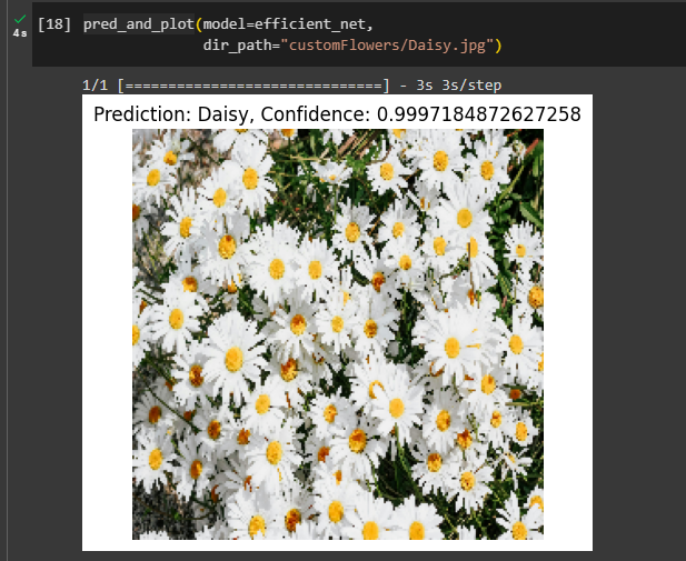
Daaamn, that's a really high confidence from our EfficientNet model, but the image is of a decent quality as well.
Dandelion Flower Prediction
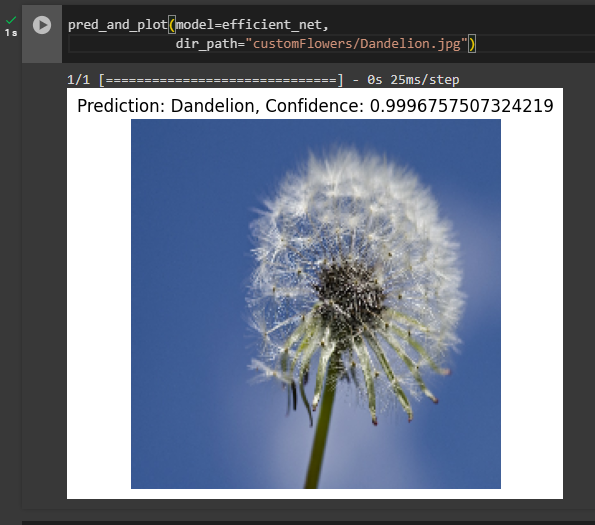
That's another great prediction - I mean I would be surprised if the probability was any lower, since the image is of great quality once again :D Let's now use an image with some noise to make it at least a bit more difficult for our Net.
Lavender Flower Prediction
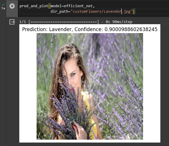
Got it right again, but the confidence dropped by around 9 percentage points because of noise in the image :D.
Lilly Flower Prediction
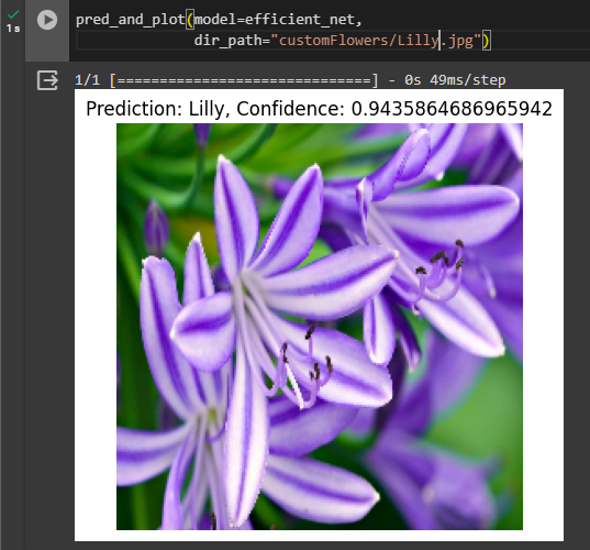
Yup, that is another one great guess... Bet our net really learned the Lillies well...
Lotus Flower Prediction
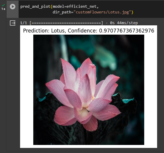
Even better than the previous one! Flawlessly once again! Let's make it harder for the model.
Orchid Flower Prediction
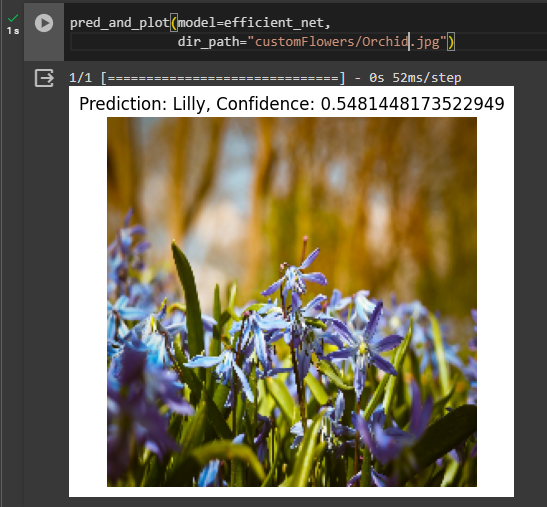
Finally, got him to make a mistake! I chose this image, because to me, it imitates Lilly, Lavender, and Orchid at the same time. And this is where our Net made a mistake.
The confidence is pretty low too, so apparently it had trouble deciding on the particular class... I guess this is some basis, where we could potentially start to improve our model. Some failure is important to see as well... Let's go on to the last three predictions...
Rose & Sunflower & Tulip Predictions
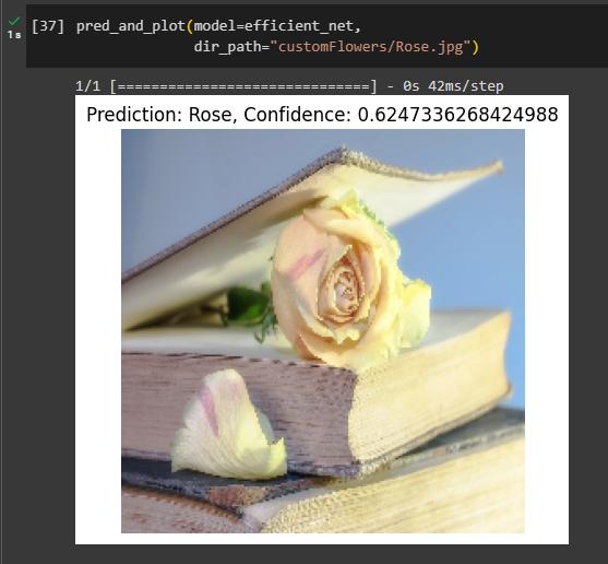
Got it correctly! Confidence isn't high because there's, again, some random noise in the image like the book. But I'm glad he managed to classify it correctly nonetheless :D
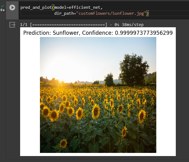
Unmatched confidence 💪 The image is of a relatively decent quality as well.
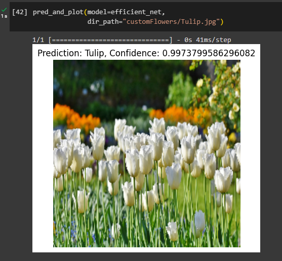
Once again - some custom Tulip image ain't got nothing on our great EfficientNetB0 model... I'm pretty satisfied with the results :D
Conclusion
I'm pretty satisfied with the results of our EfficientNet. It was able to correctly classify nearly all images - it struggled with some unclear/noisy data. I guess that could be some starting base, where we could try to improve the model. I didn't yet dive into the concept of fine-tuning models, so I'm really proud of the results so far :D
It was my first blog ever on the Hashnode, so any feedback will be appreciated 🤝